Creating Curves in RatesLib Versus QuantLib
The purpose of this short blog post is to outline the differences in creating yield curves between RatesLib and QuantLib.
QuantLib
Consider the objective of bootstrapping two deposit rates using QuantLib, which is shown below:
# Set reference date
ql_date = ql.Date("2023-01-11", "%Y-%m-%d")
ql.Settings.instance().evaluationDate = ql_date

# Define all the properties of the instrument
rates = [3.218, 3.330]
maturity= ['3M', '6M']
bor_calendar = ql.TARGET()
fixing_day = 0
convention = ql.ModifiedFollowing
day_counter= ql.Actual360()

# Create the DepositRateHelper
helpers = [ql.DepositRateHelper(ql.QuoteHandle(ql.SimpleQuote(r/100.0)),
                    ql.Period(t),
                    fixing_day,
                    calendar,
                    convention,
                    day_counter) for r, t in zip(rates,maturity)]
Given the first deposit, QuantLib will aim to solve the following optimization problem when solving for the term structure:
\[\textrm{min}_{df} \ \textrm{rate} - (\frac{df(t_2)}{df(t_1)} - 1)/(t_2-t_1).\]Where
- $df$ is a function returning the discounting factor for a corresponding maturity $t_i$.
- $t_1$ will be the adjusted reference date if it is on a holiday and $t_2$ will be the adjusted maturity date.
- rate is the input quote (mid-market rate).
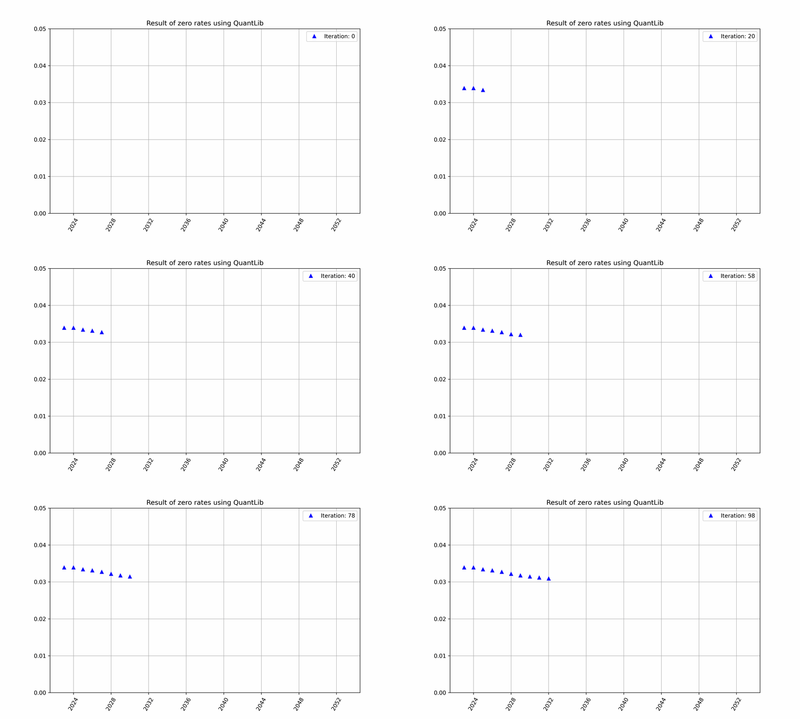
Initially the function $df$ will contain guesses which will iteratively converge to the true values using the equation above for each helper, this is highlighted in Figure 1.

Figure 1: An example of iterative bootstrapping for a different set of instruments.
RatesLib
Finding the term structure in RatesLib differs from how QuantLib does it. As stated in the documentation of RatesLib it is said that the solver will find the solution of the following equation:
\[\textrm{min}_v \ f(\vec{v}, \vec{S}) = \textrm{min}_v \ (\vec{r}(\vec{v}) - \vec{S})W(\vec{r}(\vec{v}) - \vec{S})^T\]Where
- $\vec{v}$ corresponds to the input discount factors.
- $\vec{r}$ are the zero rates given by the instruments by using $\vec{v}$.
- $\vec{S}$ is the input instrument’s rates, similiar to our deposit’s rates above for QuantLib.
- $W$ is the diagonal matrix of weights.
Thus the solver will
- Use $\vec{v}$ to find $\vec{r}$.
- Apply an algorithm (e.g., Gauss-Newton) for one iteration of the minimization problem.
- Update $\vec{v}$ which in turn will update $\vec{r}$.
- Repeat step 1,2,3 to convergence.
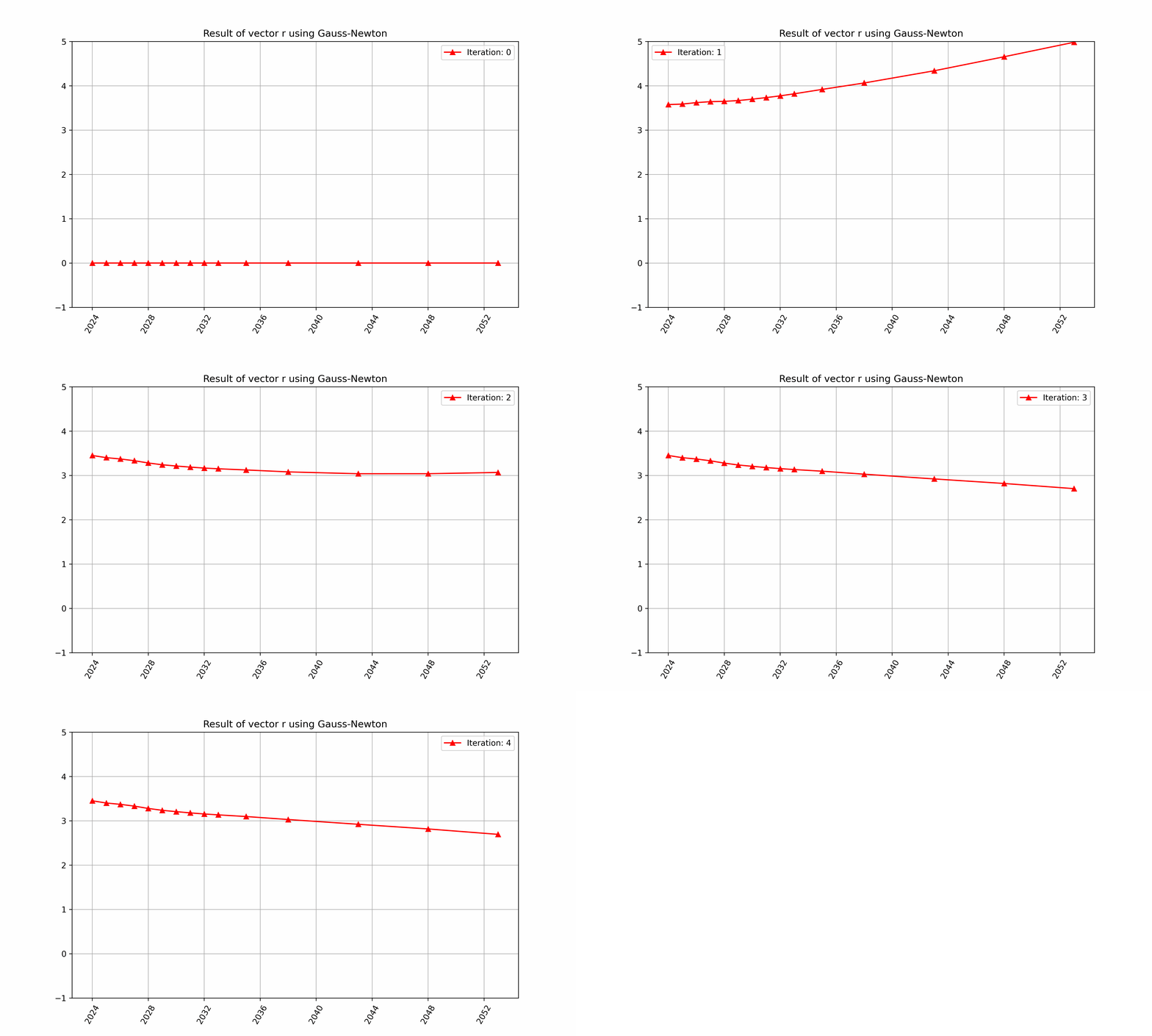
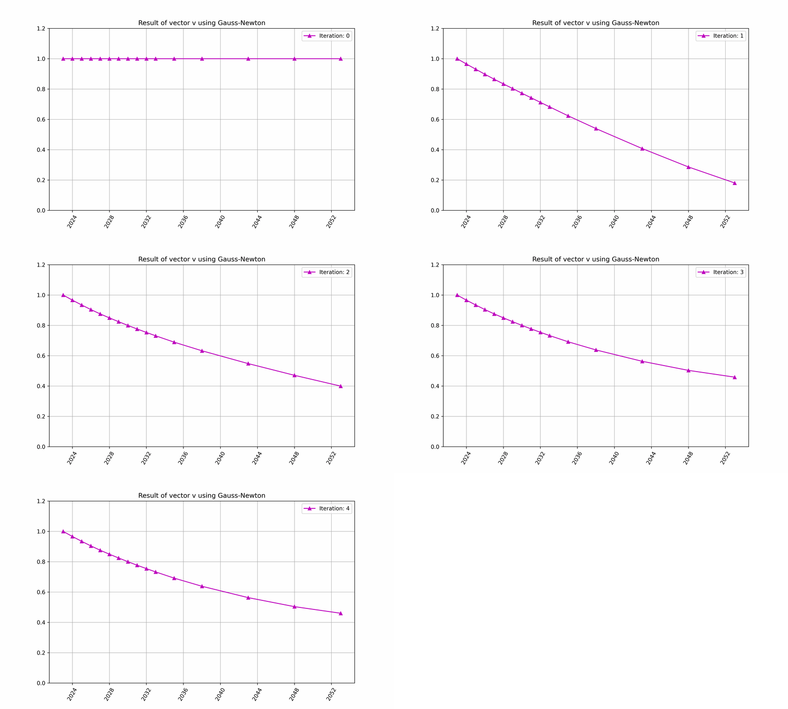
The iteration of above in RatesLib is highlighted in Figure 2 and 3.

Figure 2: An example of finding $\vec{r}$ with RatesLib.

Figure 2: An example of finding $\vec{v}$ with RatesLib.